%matplotlib inline

Utilities that assist in building USID Ancillary datasets manually

Suhas Somnath

4/18/2018

This document illustrates certain helper functions that simplify building ancillary Universal Spectroscopy and Imaging Data (USID) datasets manually

Introduction

The USID model takes a unique approach towards towards storing scientific observational data. Several helper functions are necessary to simplify the actual file writing process. In some circunstances, the data does not have an N-dimensonal form and we therefore cannot use the pyUSID.Dimension objects to define the ancillary Datasets. pyUSID.anc_build_utils is home for those utilities that assist in manually building ancillary USID datasets but do not directly interact with HDF5 files (as in pyUSID.hdf_utils).

Note that most of these are low-level functions that are used by popular high level functions in pyUSID.hdf_utils to simplify the writing of datasets.

Recommended pre-requisite reading

• Universal Spectroscopic and Imaging Data (USID) model

What to read after this

• Crash course on HDF5 and h5py

• Utilities for reading and writing h5USID files using pyUSID

Import necessary packages

We only need a handful of packages besides pyUSID to illustrate the functions in pyUSID.anc_build_utils:

• numpy - for numerical operations on arrays in memory

• matplotlib - basic visualization of data

from __future__ import print_function, division, unicode_literals
# Warning package in case something goes wrong
from warnings import warn
import numpy as np
import matplotlib.pyplot as plt
import subprocess
import sys


def install(package):
    subprocess.call([sys.executable, "-m", "pip", "install", package])
# Package for downloading online files:
# Finally import pyUSID.
try:
    import pyUSID as usid
except ImportError:
    warn('pyUSID not found.  Will install with pip.')
    import pip
    install('pyUSID')
    import pyUSID as usid

Building Ancillary datasets

The USID model uses pairs of ancillary matrices to support the instrument-agnostic and compact representation of multidimensional datasets. While the creation of ancillary datasets is straightforward when the number of position and spectroscopic dimensions are relatively small (0-2), one needs to be careful when building these ancillary datasets for datasets with large number of position / spectroscopic dimensions (> 2). The main challenge involves the careful tiling and repetition of unit vectors for each dimension with respect to the sizes of all other dimensions. Fortunately, pyUSID.anc_build_utils has many handy functions that solve this problem.

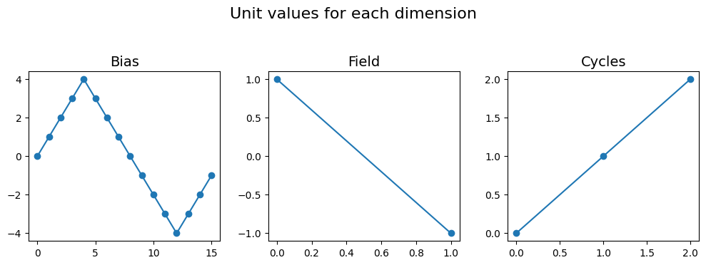
In order to demonstrate the functions, lets say that we are working on an example Main dataset that has three spectroscopic dimensions (Bias, Field, Cycle). The Bias dimension varies as a bi-polar triangular waveform. This waveform is repeated for two Fields over 3 Cycles meaning that the Field and Cycle dimensions are far simpler than the Bias dimension in that they have linearly increasing / decreasing values.

max_v = 4
half_pts = 8
bi_triang = np.roll(np.hstack((np.linspace(-max_v, max_v, half_pts, endpoint=False),
                               np.linspace(max_v, -max_v, half_pts, endpoint=False))), -half_pts // 2)
cycles = [0, 1, 2]
fields = [1, -1]

dim_names = ['Bias', 'Field', 'Cycles']

fig, axes = plt.subplots(ncols=3, figsize=(10, 3.5))
for axis, name, vec in zip(axes.flat, dim_names, [bi_triang, fields, cycles]):
    axis.plot(vec, 'o-')
    axis.set_title(name, fontsize=14)
fig.suptitle('Unit values for each dimension', fontsize=16, y=1.05)
fig.tight_layout()

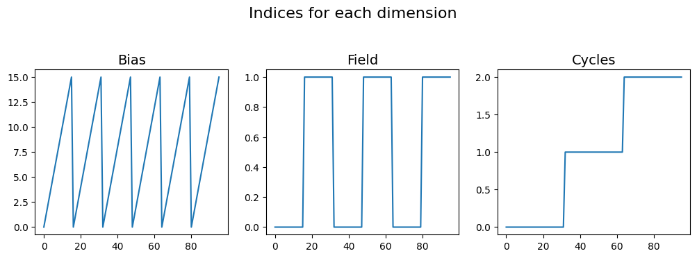
make_indices_matrix()

One half of the work for generating the ancillary datasets is generating the indices matrix. The make_indices_matrix() function solves this problem. All one needs to do is supply a list with the lengths of each dimension. The result is a 2D matrix of shape: (3 dimensions, points in Bias[16] * points in Field[2] * points in Cycle[3]) = (3, 96).

inds = usid.anc_build_utils.make_indices_matrix([len(bi_triang), len(fields), len(cycles)], is_position=False)
print('Generated indices of shape: {}'.format(inds.shape))

# The plots below show a visual representation of the indices for each dimension:
fig, axes = plt.subplots(ncols=3, figsize=(10, 3.5))
for axis, name, vec in zip(axes.flat, dim_names, inds):
    axis.plot(vec)
    axis.set_title(name, fontsize=14)
fig.suptitle('Indices for each dimension', fontsize=16, y=1.05)
fig.tight_layout()

Generated indices of shape: (3, 96)

build_ind_val_matrices()

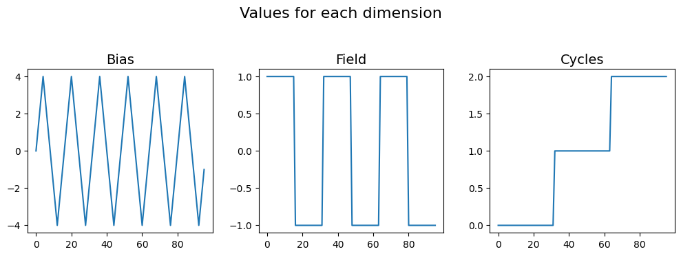
make_indices_matrix() is a very handy function but it only solves one of the problems - the indices matrix. We also need the matrix with the values tiled and repeated in the same manner. Perhaps one of the most useful functions is build_ind_val_matrices() which uses just the values over which each dimension is varied to automatically generate the indices and values matrices that form the ancillary datasets.

In order to generate the indices and values matrices, we would just need to provide the list of values over which these dimensions are varied to build_ind_val_matrices(). The results are two matrices - one for the indices and the other for the values, of the same shape (3, 96).

As mentioned in our document about the data structuring <../../data_format.html>_, the Bias would be in the first row, followed by Field, finally followed by Cycle. The plots below illustrate what the indices and values look like for each dimension. For example, notice how the bipolar triangular bias vector has been repeated 2 (Field) * 3 (Cycle) times. Also note how the indices vector is a saw-tooth waveform that also repeats in the same manner. The repeated + tiled indices and values vectors for Cycle and Field look the same / very similar since they were simple linearly increasing values to start with.

inds, vals = usid.anc_build_utils.build_ind_val_matrices([bi_triang, fields, cycles], is_spectral=True)
print('Indices and values of shape: {}'.format(inds.shape))

fig, axes = plt.subplots(ncols=3, figsize=(10, 3.5))
for axis, name, vec in zip(axes.flat, dim_names, inds):
    axis.plot(vec)
    axis.set_title(name, fontsize=14)
fig.suptitle('Indices for each dimension', fontsize=16, y=1.05)
fig.tight_layout()

fig, axes = plt.subplots(ncols=3, figsize=(10, 3.5))
for axis, name, vec in zip(axes.flat, dim_names, vals):
    axis.plot(vec)
    axis.set_title(name, fontsize=14)
fig.suptitle('Values for each dimension', fontsize=16, y=1.05)
fig.tight_layout()

Indices and values of shape: (3, 96)

create_spec_inds_from_vals()

When writing analysis functions or classes wherein one or more (typically spectroscopic) dimensions are dropped as a consequence of dimensionality reduction, new ancillary spectroscopic datasets need to be generated when writing the reduced data back to the file. create_spec_inds_from_vals() is a handy function when we need to generate the indices matrix that corresponds to a values matrix. For this example, lets assume that we only have the values matrix but need to generate the indices matrix from this:

inds = usid.anc_build_utils.create_spec_inds_from_vals(vals)

fig, axes = plt.subplots(ncols=3, figsize=(10, 3.5))
for axis, name, vec in zip(axes.flat, dim_names, inds):
    axis.plot(vec)
    axis.set_title(name, fontsize=14)
fig.suptitle('Indices for each dimension', fontsize=16, y=1.05)
fig.tight_layout()

get_aux_dset_slicing()

Region references are a handy feature in HDF5 that allow users to refer to a certain section of data within a dataset by name rather than the indices that define the region of interest.

In USID, we use region references to define the row or column in the ancillary dataset that corresponds to each dimension by its name. In other words, if we only wanted the Field dimension we could directly get the data corresponding to this dimension without having to remember or figure out the index in which this dimension exists.

Let’s take the example of the Field dimension which occurs at index 1 in the (3, 96) shaped spectroscopic index / values matrix. We could extract the Field dimension from the 2D matrix by slicing each dimension using slice objects . We need the second row so the first dimension would be sliced as slice(start=1, stop=2). We need all the colummns in the second dimension so we would slice as slice(start=None, stop=None) meaning that we need all the columns. Doing this by hand for each dimension is clearly tedious.

get_aux_dset_slicing() helps generate the instructions for region references for each dimension in an ancillary dataset. The instructions for each region reference in h5py are defined by tuples of slice objects. Lets see the region-reference instructions that this function provides for our aforementioned example dataset with the three spectroscopic dimensions.

print('Region references slicing instructions for Spectroscopic dimensions:')
ret_val = usid.anc_build_utils.get_aux_dset_slicing(dim_names, is_spectroscopic=True)
for key, val in ret_val.items():
    print('{} : {}'.format(key, val))

print('\nRegion references slicing instructions for Position dimensions:')
ret_val = usid.anc_build_utils.get_aux_dset_slicing(['X', 'Y'], is_spectroscopic=False)
for key, val in ret_val.items():
    print('{} : {}'.format(key, val))

Region references slicing instructions for Spectroscopic dimensions:
Bias : (slice(0, 1, None), slice(None, None, None))
Field : (slice(1, 2, None), slice(None, None, None))
Cycles : (slice(2, 3, None), slice(None, None, None))

Region references slicing instructions for Position dimensions:
X : (slice(None, None, None), slice(0, 1, None))
Y : (slice(None, None, None), slice(1, 2, None))

Dimension

In USID, position and spectroscopic dimensions are defined using some basic information that will be incorporated in Dimension objects that contain three vital pieces of information:

• name of the dimension

• units for the dimension

• values:

  • These can be the actual values over which the dimension was varied

  • or number of steps in case of linearly varying dimensions such as ‘Cycle’ below

These objects will be heavily used for creating Main or ancillary datasets in pyUSID.hdf_utils and even to set up interactive jupyter Visualizers in pyUSID.USIDataset.

Note that the Dimension objects in the lists for Position and Spectroscopic must be arranged from fastest varying to slowest varying to mimic how the data is actually arranged. For example, in this example, there are multiple bias points per field and multiple fields per cycle. Thus, the bias changes faster than the field and the field changes faster than the cycle. Therefore, the Bias must precede Field which will precede Cycle. Let’s assume that we were describing the spectroscopic dimensions for this example dataset to some other pyUSID function , we would describe the spectroscopic dimensions as:

spec_dims = [usid.Dimension('Bias', 'V', bi_triang),
             usid.Dimension('Fields', '', fields),
             # for the sake of example, since we know that cycles is linearly increasing from 0 with a step size of 1,
             # we can specify such a simply dimension via just the length of that dimension:
             usid.dimension.Dimension('Cycle', '', len(cycles))]

---------------------------------------------------------------------------
AttributeError                            Traceback (most recent call last)
Cell In[8], line 5
      1 spec_dims = [usid.Dimension('Bias', 'V', bi_triang),
      2              usid.Dimension('Fields', '', fields),
      3              # for the sake of example, since we know that cycles is linearly increasing from 0 with a step size of 1,
      4              # we can specify such a simply dimension via just the length of that dimension:
----> 5              usid.dimension.Dimension('Cycle', '', len(cycles))]

AttributeError: module 'pyUSID' has no attribute 'dimension'

The application of the Dimension objects will be a lot more apparent in the document about the writing functions in pyUSID.hdf_utils.

Misc writing utilities

calc_chunks()

The h5py package automatically (virtually) breaks up HDF5 datasets into contiguous chunks to speed up reading and writing of datasets. In certain situations the default mode of chunking may not result in the highest performance. In such cases, it helps in chunking the dataset manually. The calc_chunks() function helps in calculating appropriate chunk sizes for the dataset using some apriori knowledge about the way the data would be accessed, the size of each element in the dataset, maximum size for a single chunk, etc. The examples below illustrate a few ways on how to use this function:

dimensions = (16384, 16384 * 4)
dtype_bytesize = 4
ret_val = usid.anc_build_utils.calc_chunks(dimensions, dtype_bytesize)
print(ret_val)

dimensions = (16384, 16384 * 4)
dtype_bytesize = 4
unit_chunks = (3, 7)
max_mem = 50000
ret_val = usid.anc_build_utils.calc_chunks(dimensions, dtype_bytesize, unit_chunks=unit_chunks, max_chunk_mem=max_mem)
print(ret_val)

(26, 100)
(57, 224)