2D plotting utilities

Suhas Somnath

8/12/2017

This is a short walk-through of useful plotting utilities available in sidpy

Introduction

Some of the functions in sidpy.viz.plot_utils fill gaps in the default matplotlib package, some were developed for scientific applications, These functions have been developed to substantially simplify the generation of high quality figures for journal publications.

Table of contents:

• plot_map

• plot_map_stack

• plot_complex_spectra

Import necessary packages:

from __future__ import division, print_function, absolute_import, unicode_literals
import numpy as np
from warnings import warn
import matplotlib.pyplot as plt
import subprocess
import sys


def install(package):
    subprocess.call([sys.executable, "-m", "pip", "install", package])
# Package for downloading online files:
try:
    import sidpy
except ImportError:
    warn('sidpy not found.  Will install with pip.')
    import pip
    install('sidpy')
    import sidpy

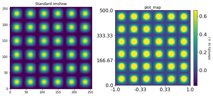
plot_map()

This function adds several popularly used features to the basic image plotting function in matplotlib including:

• easy addition of a colorbar

• custom x and y tick values

• clipping the colorbar to N standard deviations of the mean

x_vec = np.linspace(0, 6*np.pi, 256)
y_vec = np.sin(x_vec)**2

atom_intensities = y_vec * np.atleast_2d(y_vec).T

fig, axes = plt.subplots(ncols=2, figsize=(10, 5))

# Standard imshow plot for reference
axes[0].imshow(atom_intensities, origin='lower')
axes[0].set_title('Standard imshow')


# Now plot_map with some options enabled:
sidpy.viz.plot_utils.plot_map(axes[1], atom_intensities, stdevs=1.5, num_ticks=4,
                       x_vec=np.linspace(-1, 1, atom_intensities.shape[0]),
                       y_vec=np.linspace(0, 500, atom_intensities.shape[1]),
                       cbar_label='intensity (a. u.)', tick_font_size=16)
axes[1].set_title('plot_map')
fig.tight_layout()

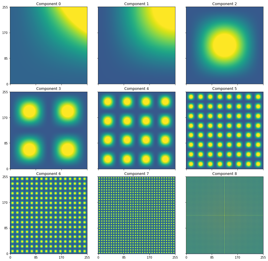
plot_map_stack()

One of the most popular operations in scientific research is the visualization of a stack of images.

This function is built specifically for that purpose.

Here we simply simulate some images using sinusoidal functions for demonstration purposes.

def get_sine_2d_image(freq):
    x_vec = np.linspace(0, freq*np.pi, 256)
    y_vec = np.sin(x_vec)**2
    return y_vec * np.atleast_2d(y_vec).T


frequencies = [0.25, 0.5, 1, 2, 4 ,8, 16, 32, 64]
image_stack = [get_sine_2d_image(freq) for freq in frequencies]
image_stack = np.array(image_stack)

fig, axes = sidpy.viz.plot_utils.plot_map_stack(image_stack, reverse_dims=False, title_yoffset=0.95)

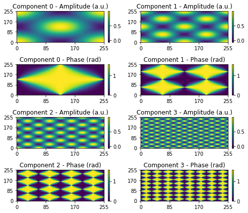
plot_complex_spectra()

This function plots the amplitude and phase components of a stack of complex valued 2D images.

Here we simulate the data using sine and cosine components

def get_complex_2d_image(freq):
    # Simple function to generate images
    x_vec = np.linspace(0, freq*np.pi, 256)
    y_vec_1 = np.sin(x_vec)**2
    y_vec_2 = np.cos(x_vec)**2
    return y_vec_2 * np.atleast_2d(y_vec_2).T + 1j*(y_vec_1 * np.atleast_2d(y_vec_1).T)


# The range of frequences over which the images are generated
frequencies = 2 ** np.arange(4)
image_stack = [get_complex_2d_image(freq) for freq in frequencies]

fig, axes = sidpy.viz.plot_utils.plot_complex_spectra(np.array(image_stack), figsize=(3.5, 3))